
ملف:Conformal map.svg

حجم معاينة PNG لذلك الملف ذي الامتداد SVG: 342 × 599 بكسل. الأبعاد الأخرى: 137 × 240 بكسل | 274 × 480 بكسل | 438 × 768 بكسل | 584 × 1٬024 بكسل | 1٬169 × 2٬048 بكسل | 535 × 937 بكسل.
الملف الأصلي (ملف SVG، أبعاده 535 × 937 بكسل، حجم الملف: 34 كيلوبايت)
| هذا ملف من ويكيميديا كومنز. معلومات من صفحة وصفه مبينة في الأسفل. كومنز مستودع ملفات ميديا ذو رخصة حرة. |
ملخص
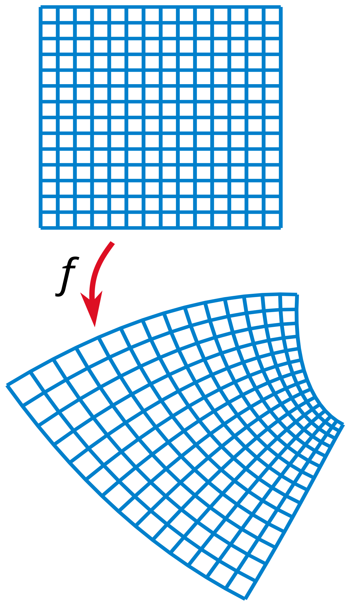
| الوصف | Illustration of a conformal map. |
| التاريخ | |
| المصدر | self-made with MATLAB, tweaked in Inkscape. |
| المؤلف | Oleg Alexandrov |
| SVG منشأ الملف | الشيفرة المصدرية لهذا الرسم المتجه صالحة. هذا الرسم المتجهي أُنشئ بواسطة Inkscape This file uses translateable embedded text. |
ترخيص
| أنا، مالِك حقوق تأليف ونشر هذا العمل، أجعله في النِّطاق العامِّ، يسري هذا في أرجاء العالم كلِّه. في بعض البلدان، قد يكون هذا التَّرخيص غيرَ مُمكنٍ قانونيَّاً، في هذه الحالة: أمنح الجميع حق استخدام هذا العمل لأي غرض دون أي شرط ما لم يفرض القانون شروطًا إضافية. |
Source code (MATLAB)
% Compute the image of a rectangular grid under a a conformal map.

function main()

   N = 15; % num of grid points
   epsilon = 0.1; % displacement for each small diffeomorphism
   num_comp = 10; % number of times the diffeomorphism is composed with itself

   S = linspace(-1, 1, N);

   [X, Y] = meshgrid(S);


   % graphing settings
   lw = 1.0;

   % KSmrq's colors
   red    = [0.867 0.06 0.14];
   blue   = [0, 129, 205]/256;
   green  = [0, 200,  70]/256;
   yellow = [254, 194,   0]/256;
   white = 0.99*[1, 1, 1];

   mycolor = blue;

   % start plotting
   figno=1; figure(figno); clf;

   shiftx = 0; shifty = 0; scale = 1;
   do_plot(X, Y, lw, figno, mycolor, shiftx, shifty, scale)

   I=sqrt(-1);
   Z = X+I*Y;

   % tweak these numbers for a pretty map
   z0 = 1+ 2*I;
   z1 = 0.1+ 0.2*I;
   z2 = 0.2+ 0.3*I;
   a = 0.01;
   b = 0.02;
   shiftx = 0.1; shifty = 1.2; scale = 1.4;
   F = (Z+z0).^2 +a*(Z+z1).^3 +b*(Z+z2).^4;
   F = (1+2*I)*F;

   XF = real(F); YF=imag(F);

   do_plot(XF, YF, lw, figno, mycolor, shiftx, shifty, scale)

   axis ([-1 1.3 -2 2]); axis off;

   saveas(gcf, 'Conformal_map.eps', 'psc2');


function do_plot(X, Y, lw, figno, mycolor, shiftx, shifty, scale)
   figure(figno); hold on;

   [M, N] = size(X);

   X = X - min(min(X));
   Y = Y - min(min(Y));

   a = max(max(max(abs(X))), max(max(abs(Y))));
   X = X/a; Y = Y/a;

   X = scale*(X-shiftx);
   Y = scale*(Y-shifty);

   for i=1:N
      plot(X(:, i), Y(:, i), 'linewidth', lw, 'color', mycolor);
      plot(X(i, :), Y(i, :), 'linewidth', lw, 'color', mycolor);
   end
%   axis([-1-small, 1+small, -1-small, 1+small]);
   axis equal; axis off;
تاريخ الملف
اضغط على زمن/تاريخ لرؤية الملف كما بدا في هذا الزمن.
| زمن/تاريخ | صورة مصغرة | الأبعاد | مستخدم | تعليق | |
|---|---|---|---|---|---|
| حالي | 21:51، 27 يناير 2008 | | 535 × 937 (34 كيلوبايت) | Oleg Alexandrov | Make arrow and text smaller |
| 03:36، 23 يناير 2008 |  | 535 × 937 (34 كيلوبايت) | Oleg Alexandrov | {{Information |Description=Illustration of a conformal map. |Source=self-made with MATLAB, tweaked in Inkscape. |~~~~~ |Author= Oleg Alexandrov |Permission= |other_versions= }} {{PD-self}} ==Source code ([[ |
استخدام الملف
الصفحتان التاليتان تستخدمان هذا الملف:
الاستخدام العالمي للملف
الويكيات الأخرى التالية تستخدم هذا الملف:
- الاستخدام في ba.wikipedia.org
- الاستخدام في ca.wikipedia.org
- الاستخدام في cbk-zam.wikipedia.org
- الاستخدام في cs.wikipedia.org
- الاستخدام في de.wikipedia.org
- الاستخدام في de.wikiversity.org
- Holomorphie/Kriterien
- Kurs:Riemannsche Flächen (Osnabrück 2022)/Vorlesung 1
- Kurs:Riemannsche Flächen (Osnabrück 2022)/Vorlesung 1/kontrolle
- Satz über die Umkehrabbildung/Implizite Abbildung/C/Zusammenfassung/Textabschnitt
- Kurs:Funktionentheorie (Osnabrück 2023-2024)/Vorlesung 4
- Kurs:Funktionentheorie (Osnabrück 2023-2024)/Vorlesung 4/kontrolle
- الاستخدام في el.wikipedia.org
- الاستخدام في en.wikipedia.org
- الاستخدام في es.wikipedia.org
- الاستخدام في fa.wikipedia.org
- الاستخدام في fi.wikipedia.org
- الاستخدام في fr.wikipedia.org
- الاستخدام في gl.wikipedia.org
- الاستخدام في he.wikipedia.org
- الاستخدام في hi.wikipedia.org
- الاستخدام في hu.wikipedia.org
- الاستخدام في hy.wikipedia.org
- الاستخدام في id.wikipedia.org
- الاستخدام في it.wikipedia.org
اعرض المزيد من الاستخدام العام لهذا الملف.