
ملف:Scattering theory illust.png
حجم هذه المعاينة: 144 × 596 بكسل. البعدان الآخران: 58 × 240 بكسل | 480 × 1٬988 بكسل.
الملف الأصلي (480 × 1٬988 بكسل حجم الملف: 49 كيلوبايت، نوع MIME: image/png)
| هذا ملف من ويكيميديا كومنز. معلومات من صفحة وصفه مبينة في الأسفل. كومنز مستودع ملفات ميديا ذو رخصة حرة. |
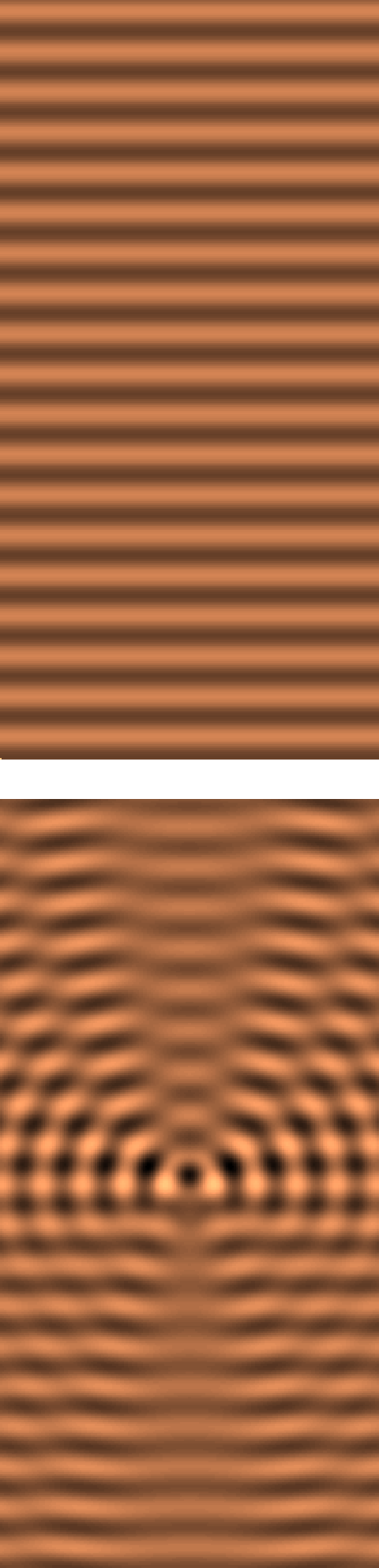
| الوصف | Illustration of en:Scattering theory. |
| التاريخ | (UTC) |
| المصدر | self-made with en:Matlab. See the source at Image:Scattering_total_field.png |
| المؤلف | Oleg Alexandrov |
.هذا الرسم المتجهي أُنشئ بواسطة MATLAB
| أنا، مالِك حقوق تأليف ونشر هذا العمل، أجعله في النِّطاق العامِّ، يسري هذا في أرجاء العالم كلِّه. في بعض البلدان، قد يكون هذا التَّرخيص غيرَ مُمكنٍ قانونيَّاً، في هذه الحالة: أمنح الجميع حق استخدام هذا العمل لأي غرض دون أي شرط ما لم يفرض القانون شروطًا إضافية. |
Source code (MATLAB)
function main(Nx, Iters)

Box_x = 3;
Scale = 0.5;
Box_y = Box_x/Scale;

%Nx = 50;
Ny = Nx/Scale;

wavenumber = 10;

XX = linspace(-Box_x, Box_x, Nx);
YY = linspace(-Box_y, Box_y, Ny);
hx = XX(2) - XX(1);
hy = YY(2) - YY(1);
[X, Y] = meshgrid(XX, YY);

Source_size  = 0.5;
Source_shift = 0;
n0=0.5;
Scatterer =  n0*sign(max(Source_size^2 - X.^2-(Y-Source_shift).^2, 0));

I = sqrt(-1);
Uinc = exp(I*wavenumber*Y);

% plot the initial planewave
figure(1); clf; hold on; axis equal; axis off; colormap copper;
Tweak=0*Uinc; Tweak(1, 1)=-2; Tweak(1, 2) = 4;
imagesc(real(Uinc)+Tweak); % a hack to have the same colormap as the images below
iter = 1;
saveas(gcf, sprintf('Scattering_frame%d_Nx%d.eps', iter, Nx), 'psc2');

%figure(3); clf; hold on; axis equal; axis off; colormap copper;
%imagesc(Scatterer);

% Approximate the Uscatter by 0
Uscatter = 0*Scatterer;

% Several iterations to improve upon the starting Born approximation
% I hope this is the right way to do things. The plotted solution looks plausible
% but I don't know if this is rigurous.

for iter=2:(1+Iters)

   % Here we use an approximate source
   Source = wavenumber^2*Scatterer.*(Uinc+Uscatter);

   % calc the solution solution to the Helmholtz equation
   Uscatter = 0*X;
   [m, n] = size(Source);
   for i=1:m
      i
      for j=1:n

	 if Source(i, j) ~= 0

	    x0 = X(i, j);
	    y0 = Y(i, j);

            % add the contribution from the current source, average over four corners of current rectangle
	    Uscatter = Uscatter ...
		+ (I/16)*(...
		   besselh(0, 1, wavenumber*sqrt((X-x0-hx/2).^2+(Y-y0-hy/2).^2) + eps)*Source(i, j) ...
		   + besselh(0, 1, wavenumber*sqrt((X-x0-hx/2).^2+(Y-y0+hy/2).^2) + eps)*Source(i, j) ...
		   + besselh(0, 1, wavenumber*sqrt((X-x0+hx/2).^2+(Y-y0-hy/2).^2) + eps)*Source(i, j) ...
		   + besselh(0, 1, wavenumber*sqrt((X-x0+hx/2).^2+(Y-y0+hy/2).^2) + eps)*Source(i, j))*hx*hy;
%Uscatter = Uscatter +(I/4)*besselh(0, 1, wavenumber*sqrt((X-x0).^2+(Y-y0).^2) + eps)*Source(i, j)*hx*hy;
	 end

      end
   end

   Utotal = Uinc + Uscatter;

   figure(1); clf; hold on; axis equal; axis off; colormap copper;
   imagesc(real(Utotal));
   saveas(gcf, sprintf('Scattering_frame%d_Nx%d.eps', iter, Nx), 'psc2');
end

|
هذه math الصورة / الصورتان باستعمال رسومات متجهية ملفات رسوميات شعاعية.
It is recommended to name the SVG file "Scattering theory illust.svg" - then the template Vector version available (or Vva) does not need the new image name parameter.
|
تاريخ الملف
اضغط على زمن/تاريخ لرؤية الملف كما بدا في هذا الزمن.
| زمن/تاريخ | صورة مصغرة | الأبعاد | مستخدم | تعليق | |
|---|---|---|---|---|---|
| حالي | 04:44، 8 يوليو 2007 | 480 × 1٬988 (49 كيلوبايت) | Oleg Alexandrov | Tweak | |
| 04:40، 8 يوليو 2007 | 480 × 2٬054 (49 كيلوبايت) | Oleg Alexandrov | {{Information |Description=Illustration of en:Scattering theory. |Source=self-made with en:Matlab. See the source at Image:Scattering_total_field.png |Date=03:21, 8 July 2007 (UTC) |Author= Oleg Alexandrov }} {{PD- |
استخدام الملف
الصفحة التالية تستخدم هذا الملف:
الاستخدام العالمي للملف
الويكيات الأخرى التالية تستخدم هذا الملف:
- الاستخدام في ca.wikipedia.org
- الاستخدام في en.wikipedia.org
- الاستخدام في es.wikipedia.org
- الاستخدام في pa.wikipedia.org
- الاستخدام في pt.wikipedia.org